Reviving 65 Guitars, and the Silent Ones Among Them

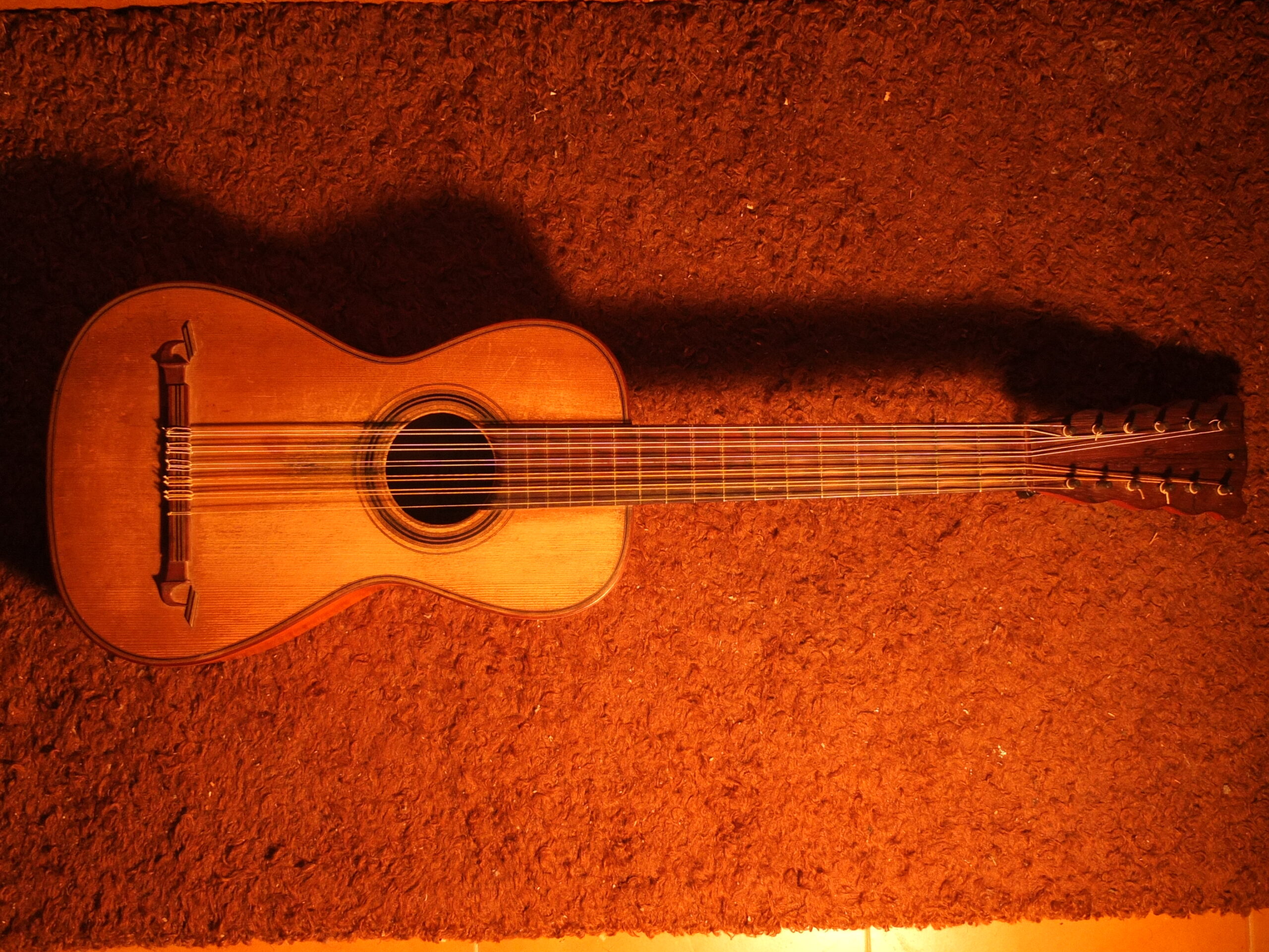
(image credit: Robert Mores, made available via his Zenodo repo)
When you pluck a classical guitar, very little of what you hear is the string. The string fixes the pitch and the timing, but almost everything that makes one guitar sound unlike another happens afterwards: the vibration crosses the bridge into the body, the body resonates, and the air carries it to you. Capture that chain faithfully, and you have captured the instrument. This project does it for sixty-five guitars at once — and for some of them, the captured version is the only one that can still be played.
This project builds directly on the Archive for the acoustical documentation of classical Spanish, flamenco and romantic guitars compiled by Robert Mores (Zenodo, 2021), which provides the bridge-mobility measurements and body radiation transfer functions for all sixty-five instruments. None of what follows would be possible without it.
A collection, and what it can no longer do
The instruments come from a public dataset assembled by Robert Mores: impulse-response measurements of sixty-five classical and flamenco guitars, their making dates running from 1803 to 2018. It is a remarkable cross-section of two centuries of lutherie — early romantic instruments by Pagés and Munoa, four originals by Antonio de Torres, the maker who effectively defined the modern classical guitar, concert instruments by Fleta, Ramírez and Bellido, flamenco blancas and negras by Conde and Reyes. They were measured between 2018 and 2019 across seven sites in Spain and Germany: luthiers’ studios in Granada, the Museu de la Música in Barcelona, an anechoic chamber in Hamburg, and the private collection of José Romanillos. They are not a uniform set: scale lengths run from 551 to 668 mm and total weights from under 700 g to more than 1750 g, so a single string model has to sit on sixty-five quite different bodies.
Some of these guitars are, for practical purposes, silent. The Torres and Pagés originals in Barcelona are tuned to historical pitch and effectively never played; several of the Romanillos early romantics have no strings at all or have deteriorated beyond being strung. For an instrument like that, the measured impulse response is not a convenience — it may be the last reliable record of how the thing actually behaved as a sounding object. That is the conviction running through the rest of NEMUS: that the sound of an instrument is part of what a collection holds, and that it can be preserved by measurement and model rather than by playing the original to pieces. Here the idea simply runs at scale — sixty-five instruments instead of one.
What a measurement contains
A guitar, for our purposes, is three things that talk to each other: a string that vibrates, a body that the string drives through the bridge, and the air that the body radiates into. The useful fact is that the body and the air are linear — double the force, and you double the response — and a linear system can be written as a sum of modes, each a damped resonance with a frequency, a decay rate, and a weight.
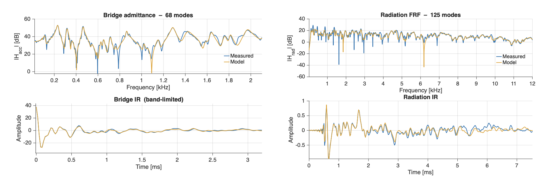
Each guitar in the dataset was struck at the bridge with a miniature impulse hammer while accelerometers on the bridge and microphones above the soundboard recorded the response. From force and response we form a frequency response function in the standard way,
\[ H(\omega)=\frac{Y(\omega)\,\overline{F(\omega)}}{|F(\omega)|^{2}}, \]
and from it we read off the body’s resonances. The bridge compliance — how readily the body yields when the string pushes on it — is written as a sum of modal contributions,
\[ H_b(\omega)=\sum_{j=1}^{J}\frac{\beta_j}{(\omega_j^{b})^{2}-\omega^{2}+2\,i\,\sigma_j^{b}\,\omega}, \]
each term a resonance with its own frequency \(\omega_j^{b}\), damping \(\sigma_j^{b}\), and weight \(\beta_j\). Fitting this sum to the measurement — peak-picking the response, estimating each peak’s bandwidth from its \(-3\) dB width, then solving a regularised least-squares problem for the weights — is the whole of the extraction. We do the same for the bridge-to-air radiation path, separately for the bass and treble sides so the final sound can be rendered in stereo. This is the part of the instrument we take directly from the data. Everything that makes a Torres a Torres and a Conde a Conde is in those numbers.

The string is the hard part
We model the string rather than measure it, and modelling it honestly is where the difficulty lies. The transverse displacement \(u(x,t)\) obeys
\[ \mu\,\partial_t^{2}u = T_0\,\partial_x^{2}u – EI\,\partial_x^{4}u – \mu\sigma\,\partial_t u + \mathcal{F}(\partial_x u) + \delta_e f_e + \delta_b F_b, \]
a stiff, damped string of mass density \(\mu\) and tension \(T_0\), driven by the pluck \(f_e\) at one point and the bridge reaction \(F_b\) at another. The term that causes the trouble is \(\mathcal{F}\), the nonlinear restoring force, which depends on the local slope \(\zeta=\partial_x u\). Under a gentle pluck a string behaves almost linearly, but a real, firm pluck does not: the tension itself rises as the string stretches, the pitch bends downward as the note decays, and energy leaks into partials that were not there at first — the faint phantom tones that give a hard-plucked string its life.
Keeping the geometry exact, the elastic energy stored per unit length is
\[ \mathcal{V}(\zeta)=\frac{G}{2}\left(\sqrt{1+\zeta^{2}}-1\right)^{2}, \qquad G = EA – T_0, \]
and it is this square-root strain — not the spatially averaged approximation of the simpler Kirchhoff–Carrier model — that produces those effects. The honesty costs something. With \(\mathcal{V}\) in the equation, a guaranteed-stable integrator has traditionally meant an implicit solver: an equation solved iteratively at every one of the forty-eight thousand samples that make up a second of audio. Multiply that by six thousand notes, and the cost is no longer academic.
A single scalar that carries the nonlinearity
The way out is a small and rather elegant trick. Because the string’s nonlinear energy
\[ \phi_{\rm nl}=\int_0^{L}\mathcal{V}(\partial_x u)\,\mathrm{d}x \ \ge\ 0 \]
is always positive, we may take its square root and treat that square root as a new unknown — a single scalar that rides along with the simulation,
\[ \psi \,\triangleq\, \sqrt{2\,\phi_{\rm nl}+\varepsilon}, \]
with \(\varepsilon\) a tiny constant that keeps the definition well posed. Differentiating, the nonlinear force factorises neatly as \(\psi\,g\) for a known gradient field \(g\), and the equations of motion become
\[ \mu\,\partial_t^{2}u = \mathcal{L}u – \psi\,g + \delta_e f_e + \delta_b F_b, \qquad \dot\psi = \langle g,\,\dot u\rangle, \]
where \(\mathcal{L}\) is the linear part of the operator. This system is exactly equivalent to the original, but it is now linear in the unknowns \(u\) and \(\psi\): the entire nonlinearity has been packed into one scalar — the Scalar Auxiliary Variable, or SAV — that simply evolves alongside the string. Its energy
\[ \mathfrak{H}=\tfrac12\,\dot{\mathbf{y}}^{\top}\dot{\mathbf{y}} + \tfrac12\,\mathbf{y}^{\top}\boldsymbol{\Omega}^{2}\mathbf{y} + \tfrac{\psi^{2}}{2} \ \ge\ 0 \]
is non-negative by construction, which is exactly what guarantees that an unforced solution cannot blow up.
What remains to solve at each step is therefore a linear system, and the only things complicating it — the bridge coupling and the scalar \(\psi\) — each enter as a rank-one change to an otherwise diagonal matrix. A rank-one change has a closed-form inverse, the Sherman–Morrison identity,
\[ \left(\mathbf{D}+\mathbf{f}\,\mathbf{v}^{\top}\right)^{-1} = \mathbf{D}^{-1} – \frac{\mathbf{D}^{-1}\mathbf{f}\,\mathbf{v}^{\top}\mathbf{D}^{-1}}{1+\mathbf{v}^{\top}\mathbf{D}^{-1}\mathbf{f}}, \]
so two applications — one for the bridge, one for the nonlinearity — give the whole update explicitly, at a cost that grows only linearly with the number of modes. In plain terms: a fully nonlinear string, coupled to a measured body, that runs about as cheaply as a linear one.
The scalar does need watching. Left alone, it can drift away from the energy it is meant to track, or flip sign, and either fault surfaces as audible misbehaviour. Two small corrections keep it honest — one nudging it back toward its true value at each step, the other forbidding the sign flip — and with those in place, the scheme is both stable and clean.
Putting the guitar back together
With the string solved and the body taken from measurement, the rest is assembly. Each body mode behaves as a driven oscillator,
\[ m_j^{b}\left(\ddot r_j + 2\sigma_j^{b}\,\dot r_j + (\omega_j^{b})^{2} r_j\right) = -\beta_j\,F_b, \]
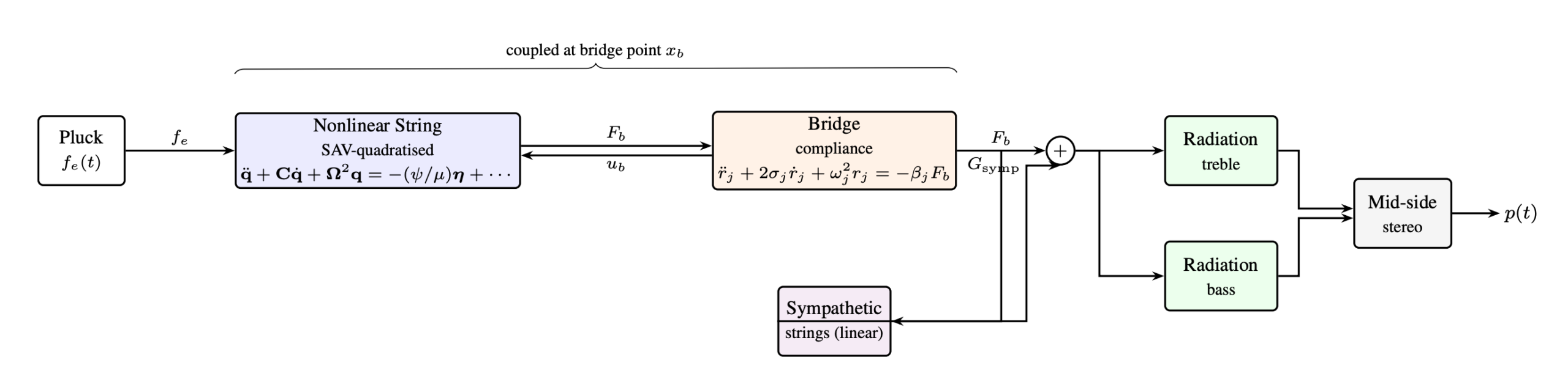
driven by the bridge force \(F_b\), which is itself fixed by demanding that the string and the bridge move together at the contact point near the string’s end. The bridge force then feeds the radiation filters, a pole–residue model of the path from bridge to air,
\[ H_{\rm rad}(\omega)=\sum_{l}\frac{b_l}{i\omega-p_l}+\frac{\bar b_l}{i\omega-\bar p_l}, \qquad p_l=-\sigma_l^{r}+i\,\omega_l^{r}, \]
fitted for the bass and treble sides and combined through mid-side processing into a stereo image. The five strings you did not pluck are still there, ringing in sympathy, so they are included too, as a bank of linear resonators driven by the same bridge force. The result is a single signal chain that takes a pluck in and outputs a stereo guitar tone.
Six thousand plucks
For each of the sixty-five guitars, we synthesised every note up to the first fifteen frets on all six strings — around six thousand two hundred plucked tones in all, written out as a library of samples. The strings follow a standard D’Addario EJ45 set, the nonlinear coupling is capped at 5 kHz to save computation with no audible loss, and everything runs at 48 kHz. They are not interchangeable. Pitch glide and phantom partials appear as they should under a firm pluck, but the body resonances underneath them are specific to each instrument, and the differences are audible from one guitar to the next. With the silent instruments, you can hear the collection’s range in a way that no other form can.
A note is not yet cheap enough to play live — a five-second tone takes a fraction of a second to compute, and the full library took a few hours on an ordinary workstation — but nothing about the method stands in the way of a real-time version, which is the obvious next build.
You can hear a selection on our guitar synthesis playlist.
Open all the way through
This project exists because someone else made their measurements public. Robert Mores documented sixty-five guitars — many of them rare, several of them silent — and placed the data on Zenodo for anyone to use; without that act, there would be nothing here to model. It would be a poor sort of gratitude to lock the result away. So the outputs go back out the same way: the sample library, the modal parameters fitted for each instrument, and the extraction and synthesis code are released openly on the project’s repositories, under licences that let other luthiers, researchers and composers take them and build on them.
The reasoning is the same one that runs through the rest of NEMUS, from the openly published hardware and software of the Trasuntino keyboard to the datasets and DOIs behind every result. A preserved sound that no one can reach is not really preserved. The whole point of turning a silent guitar into numbers is lost if the numbers stay on a private disk: they have to be copyable — open enough that the next person can carry them further than we did. Open science is not a courtesy added at the end here; it is the mechanism by which a measurement becomes shared heritage rather than a private souvenir.
What a measurement can become
The thread running through this, as through the harpsichord work before it, is a single shift in what we take a recording to be. An impulse response is usually thought of as a fixed snapshot — the sound of one strike, one instrument, one moment. Coupled to a physical model, it becomes something closer to an instrument in its own right: not a recording of a guitar being played, but the guitar itself, available to be played again, including the ones that can no longer be strung. Sixty-five of them now exist in that second form. The work still to do is concrete enough — a real-time engine, listening tests against recordings of the same instruments, and strings that share a bridge and feed one another — but the library is already there to be heard.
The guitar measurements are drawn from the publicly available dataset of Mores. The method is described in full in the accompanying paper, presented at the 29th International Conference on Digital Audio Effects (DAFx), Cambridge, MA, September 2026.