The Physics of a Plucked String — From Equations to Real-Time Sound Synthesis
By Riccardo Russo, Craig J. Webb, Michele Ducceschi & Stefan Bilbao.
Based on: "Convergence analysis and relaxation techniques for modal scalar auxiliary variable methods applied to nonlinear transverse string vibration," Proc. Mtgs. Acoust. 56, 035007 (2025) doi.org/10.1121/2.0002073. [POMA Student Paper Competition Winner]
What makes a plucked string sound like a plucked string, and not just a sine wave? The answer lies in the physics of vibration — and recreating that physics inside a computer faithfully enough to fool the ear is harder than it sounds. This post walks through how this challenge was tackled, developing a real-time algorithm for nonlinear string simulation — demonstrated through a virtual harpsichord prototype with a physical keyboard.
Simulating a String: How It's Done
Every physical simulation starts with a mathematical model. For a vibrating string, that model is a Partial Differential Equation (PDE) — an equation describing how the string's displacement changes across both space and time simultaneously, encoding the string's tension, mass, and stiffness.
A computer cannot solve a continuous equation directly, so the first step is spatial discretisation: converting the PDE into a system of time-dependent Ordinary Differential Equations (ODEs) by breaking the string into a finite set of components. These ODEs are then stepped forward 44,100 times per second by a time integrator to produce audio.
There are two main strategies for spatial discretisation:
Grid-based (FDTD): place a fine grid of points along the string and approximate spatial derivatives as differences between neighbouring values. Intuitive, but with a catch — the spatial grid and the time step are coupled for stability, so a finer spatial grid forces a higher sample rate. High-frequency components also tend to travel at slightly wrong speeds on the grid, an artefact called numerical dispersion.
Modal synthesis: instead of a grid, decompose the string's motion into its natural vibration modes — the fundamental frequency, the second harmonic, and so on. This requires solving an eigenvalue problem beforehand to compute the mode shapes and their frequencies, making it more involved to set up than FDTD. However, each mode then evolves as an independent oscillator with its own exact frequency, and space and time sampling are decoupled: more modes can be added without increasing the sample rate, and the exact integrator per mode eliminates numerical dispersion. Applying physically accurate, frequency-dependent damping is also straightforward — each mode simply gets its own decay rate.
In practice, the simulation tracks the amplitude of each mode rather than displacement at hundreds of grid points. At every time step, the nonlinear force is computed, projected onto the modal basis, and used to update each mode's amplitude independently, before reconstructing the string displacement for audio output.
The Role of Nonlinearity
For small amplitudes, a string behaves almost linearly: each harmonic vibrates independently at a fixed frequency. But real strings — especially when plucked firmly — do not stay in this comfortable regime. As amplitude grows, the string stretches significantly, and that stretching feeds back into its tension. This geometric nonlinearity has direct perceptual signatures: the pitch starts slightly sharp and gradually settles into tune — the characteristic pitch glide of a hard pluck — and the sound becomes spectrally richer over time as energy flows between harmonics. Neither effect is reproducible with a linear model.
The most complete description of these effects is the geometrically exact string model, derived from a full 3D treatment of string motion. It accounts for both transverse and longitudinal vibration and their coupling. This model is, however, computationally expensive. A more tractable form is obtained by Taylor-expanding its nonlinear potential and truncating at third order, which yields a single transverse equation with a cubic nonlinearity in the string slope. This cubic model retains the essential physics — pitch glide and spectral enrichment — while discarding longitudinal motion, reducing the problem to one equation and making real-time simulation feasible.
Capturing this correctly requires solving a significantly more complex PDE at every time step. But doing so efficiently and stably is where the real challenge lies.
The Stability Problem: Explicit, Implicit, and the SAV Trick
The standard approach to guaranteeing stability in nonlinear simulations is the energy method: design the numerical scheme so that it conserves or dissipates a discrete analogue of physical energy. For nonlinear systems, this usually leads to one of the following trade-offs:
| Scheme type | How it works | Real-time? |
|---|---|---|
| Fully implicit | Solves a nonlinear equation per time step (Newton-Raphson) | NO |
| Linearly implicit | Inverts a full matrix per time step | NO (usually) |
| Explicit | Computes the next state directly — fast, but unstable for nonlinear systems | YES |
Neither implicit approach is practical for real-time synthesis at 44,100 Hz on a consumer laptop. This is where the Scalar Auxiliary Variable (SAV) method comes in. SAV introduces a single extra variable — proportional to the square root of the nonlinear potential energy — and rewrites the equations so that the update is fully explicit and provably energy-stable.
Taming a Misbehaving Variable
SAV has many advantages, but at standard audio sample rates (44,100 Hz) a serious problem emerges: the auxiliary variable can spontaneously flip sign, causing the nonlinear force to point in the wrong direction. This compromises the numerical solution entirely: the simulated string no longer behaves physically, and the audio output is corrupted by noise.
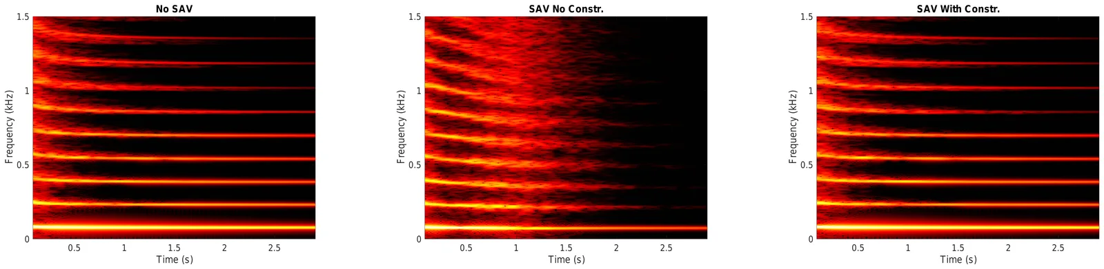 |
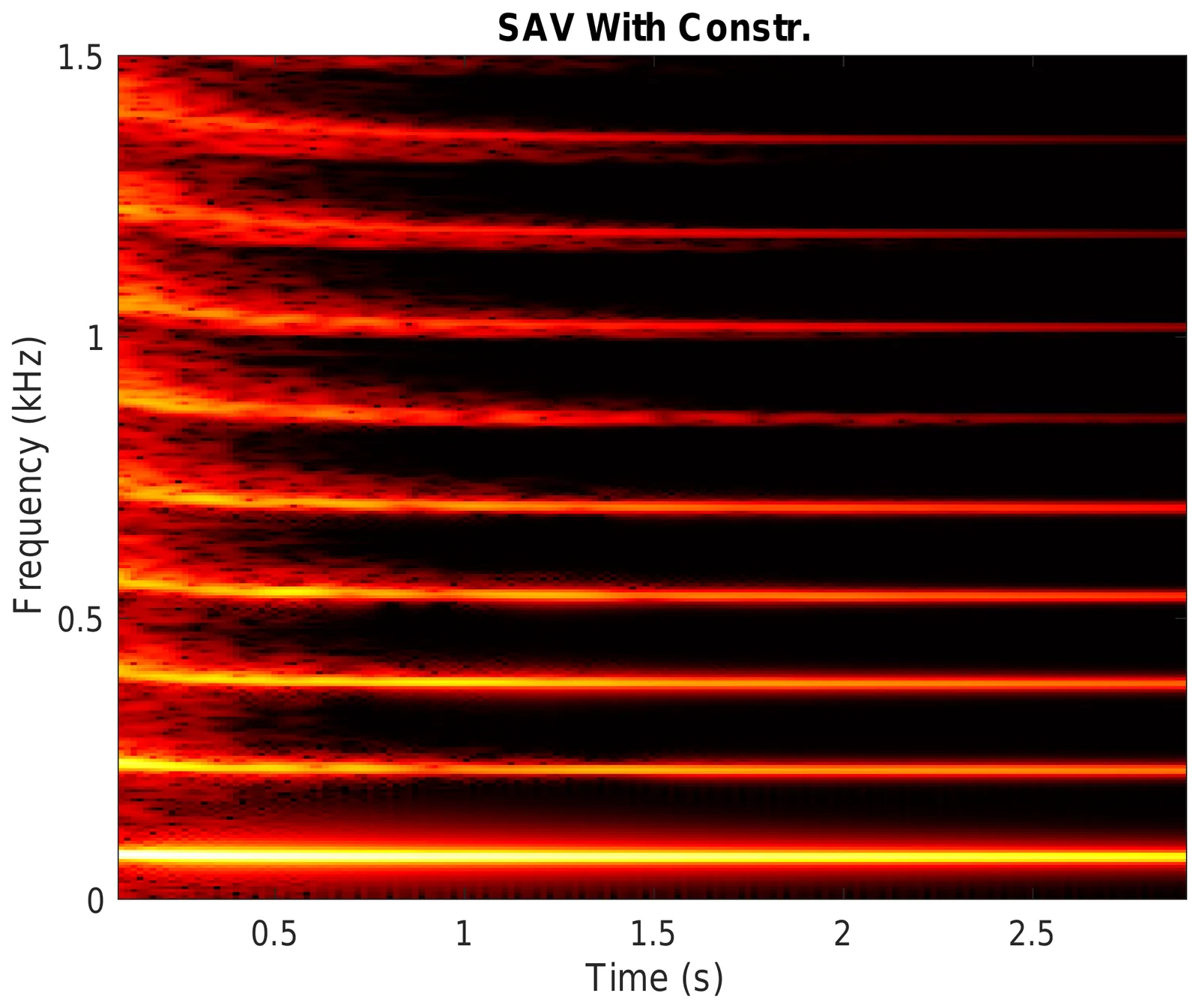
|---|
| Figure 1 Spectrograms of the plucked string simulation. Left: high-fidelity reference. Centre: SAV at audio rate without the constraint — overtones collapse into noise. Right: SAV with the constraint — the characteristic pitch glide reappears. |
The fix, borrowed from collision modelling, is a soft constraint on the auxiliary variable. At each time step, the algorithm checks whether the variable is about to go negative and, if so, computes a single scalar scaling factor to correct it. The overhead is negligible, but the improvement is dramatic.
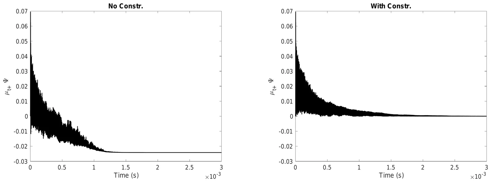 |
|---|
| Figure 2 The auxiliary variable without the constraint (left) dips below zero, corrupting the simulation. With the constraint active (right), it stays positive throughout. |
From Algorithm to Instrument: The Augmented Harpsichord
The efficiency of the modal SAV method makes it practical as the core of a real instrument. The algorithm was embedded into a virtual harpsichord plugin running in a standard DAW, connected to a physical three-key harpsichord prototype built by an expert instrument maker. The keyboard is augmented with optical and force-sensitive sensors that track each jack's displacement and keystroke velocity, triggering MIDI events and plucking the virtual string. For more info, see the paper by Matthew Hamilton, Riccardo Russo, Craig Webb and Michele Ducceschi: "A two-register haptic interface for articulated control of harpsichord physical models", Proc. Forum Acusticum (2025). doi.org/10.61782/fa.2025.0046.
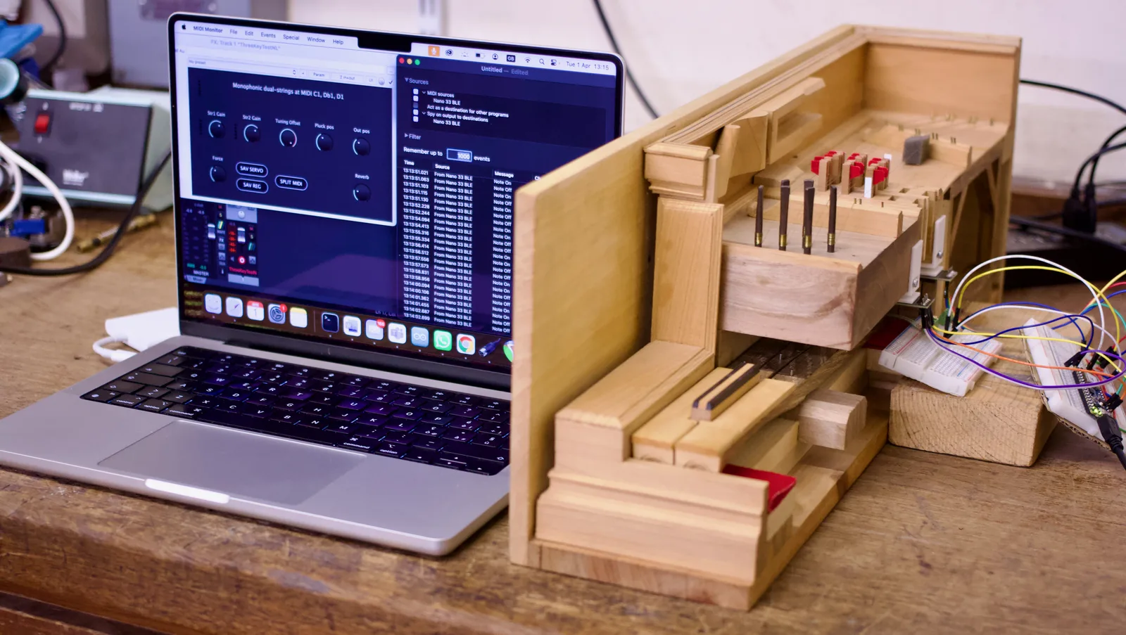 |
|---|
| Figure 3 The complete hybrid harpsichord setup: a sensor-augmented mechanical keyboard connected to a laptop running the virtual instrument. |
The simulation engine is openly available at github.com/Nemus-Project/modal-harpsichord.